The loss function for language modeling, slowly. Where the temperature knob actually lives.
Prerequisites·None
—Modalities
Narration · Module 10
Softmax + CE
0:00 / –:––
§ 01
What problem they solve
The big picture
The output head must answer one question: what word comes next?
After the transformer processes your input through N attention blocks, you have a vector of numbers (the hidden state). But you need a word — not a vector. Two mathematical tools bridge this gap every single time the model generates a token: softmax converts raw scores into a proper probability distribution, and cross-entropy measures how wrong that distribution was during training. Every word you have ever seen from ChatGPT, Claude, or Llama came through these two functions.
§ 02
Softmax — live playground
Softmax
Softmax turns raw scores into a probability distribution
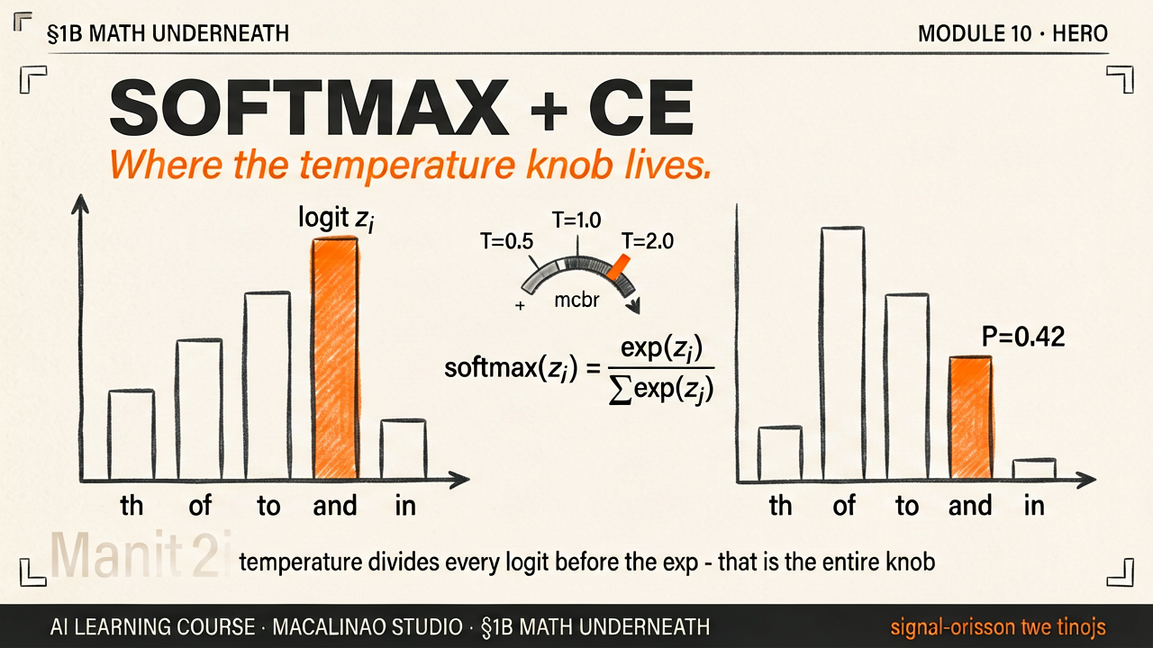
The model produces one raw score (logit) per vocabulary word — but raw scores can be any number: positive, negative, very large, very small. Softmax converts them to a clean probability distribution where every number is between 0 and 1, and all numbers sum to exactly 1. The formula: for each logit zᵢ, compute e^zᵢ / Σ(e^zⱼ for all j). Try dragging the sliders below — watch the bars respond instantly.
Why e^x — why not just normalize?
You could divide each score by the sum (like a simple ratio). But e^x does something better: it amplifies differences. If one logit is 3 and another is 1, their ratio is 3:1 — but e³:e¹ = 20:2.7 ≈ 7.5:1. The exponential makes the most confident prediction stand out more sharply, while never allowing any probability to reach exactly 0. Every word stays in the game — just with a very tiny probability.
What "probability distribution" means
A probability distribution is a list of numbers that all add up to 1.0. If the model assigns probability 0.7 to "cat", that means: if you let this model pick a word thousands of times from this exact state, about 700 out of 1,000 times it would choose "cat". Softmax guarantees this mathematical property — the output is always a valid distribution, regardless of what the raw logits look like.
Numerical stability trick — subtract the max
Real implementations use a small but critical fix
If a logit is very large (e.g. 1,000), computing e^1000 overflows to infinity on any computer. Real implementations first subtract the maximum logit from all logits before exponentiating: softmax(z)ᵢ = e^(zᵢ−max(z)) / Σe^(zⱼ−max(z)). This produces exactly the same probabilities — because subtracting a constant from all logits cancels out — but prevents numerical overflow. This trick is in every deep learning framework.
§ 03
Temperature
Temperature
Temperature controls how "confident" the distribution looks
Before applying softmax, every logit is divided by a temperature value T. At T=1 (default), softmax runs normally. At T<1, logits get amplified — the distribution sharpens into a spike and the model becomes very "decisive." At T>1, logits get compressed — the distribution flattens and the model becomes more random and "creative." This is the single number behind every "creativity" slider you've seen in AI tools.
Low T — code generation
When writing code, you want predictable, correct syntax. Temperature 0.1–0.4 makes the model focus on the single most-likely next token. In most code generators, there is exactly one right way to close a bracket or continue a function signature. Low temperature exploits this — the model acts almost deterministically.
High T — creative writing
When writing a poem or brainstorming, you want surprising word choices. Temperature 0.8–1.2 flattens the distribution so lower-probability (unexpected) words get a real chance of being selected. This is why "creative mode" in LLM tools tends to produce more vivid, unusual language — the math of temperature makes it genuinely sample from the long tail.
Top-p sampling (nucleus sampling)
A complement to temperature, not a replacement
Top-p sampling (Holtzman et al. 2020) takes the smallest set of tokens whose cumulative probability exceeds p (e.g. p=0.9), then samples only from that set. This adapts dynamically — when the model is confident, the nucleus is small (just a few words). When uncertain, the nucleus is large (many plausible words). In practice top-p is used together with temperature: temperature shapes the distribution, then top-p truncates its tail. The modern sampler stack also includes min-p, top-k, and repetition penalties — and reasoning models often ship with fixed recommended temperatures rather than exposing a free dial.
§ 04
Cross-entropy loss
Cross-entropy loss
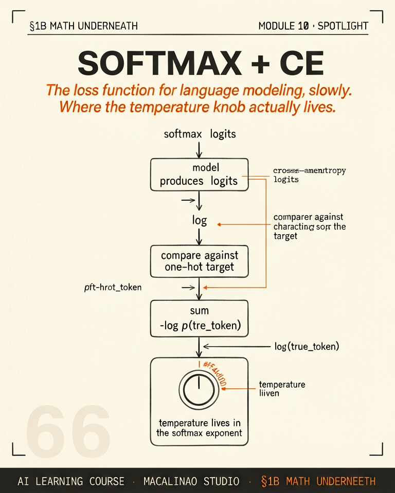
Cross-entropy measures how wrong the model's probability was
During training, we know the correct next word. Cross-entropy asks: what probability did the model assign to that correct word? The formula is simply −log(p_correct). If the model was very confident and correct (p≈1.0), the loss is near 0. If the model was confident but wrong (p≈0.0), the loss is very large. The gradient of this loss tells every weight in the network which direction to move to become more correct next time.
Why −log(p)?
The negative log has exactly the right shape: when p=1.0, −log(1)=0 (no loss — perfect). When p=0.5, −log(0.5)=0.69 (moderate loss). When p=0.01, −log(0.01)=4.6 (high loss). And as p→0, the loss approaches infinity — the model is punished extremely harshly for being confident and wrong. This asymmetry is intentional: being certain and wrong is much worse than being uncertain.
Perplexity = exp(loss)
Perplexity is the standard metric for language model quality. It equals e raised to the average cross-entropy loss. Intuitively, perplexity is "how many words was the model choosing between on average?" A perplexity of 10 means the model was effectively guessing among 10 equally likely words at each step. Lower is better. GPT-2 on Wikipedia: ~35; frontier models score far lower, though exact figures are rarely published. One caveat: perplexities are only comparable between models that share a tokenizer — different vocabularies make the per-token numbers incommensurable. A perfect model would have perplexity 1.0.
§ 05
How training uses them
Training loop
Softmax + cross-entropy together form the training loop's feedback signal
During training, the model processes a sentence and must predict each next word. Softmax converts its raw scores to probabilities. Cross-entropy compares those probabilities to the actual correct words. The resulting loss flows backwards through every weight in the network — nudging each weight slightly so the model would make a better prediction next time. Across thousands of GPUs, millions of token predictions are scored every second — though the weights themselves update only about once per second or slower, since each optimizer step batches millions of tokens. Every ability the model has came from this loop.
SFT: train on completions only
During supervised fine-tuning, cross-entropy loss is computed ONLY on the assistant's response tokens, not on the user's prompt. The model is taught to generate good answers — not to reproduce questions. This is the train_on_responses_only setting in TRL's SFTTrainer. Without this, the model wastes capacity trying to predict the prompt it was given.
Loss curves — what good training looks like
During healthy training, the loss should decrease smoothly over time. A rough heuristic for supervised fine-tuning: training loss dropping below ~0.2 can signal overfitting — the model is memorising examples rather than learning generalisable patterns. This threshold is dataset-dependent, and it does not apply to pretraining, where loss typically converges around 1.8–2.2 nats. Validation loss rising while training loss falls confirms overfitting. The ideal: both curves decrease together, converging to a low stable value.
§ 06
In attention too
Softmax in attention
Softmax appears twice — once in attention, once in the output head
Most students learn about softmax only at the output layer. But it plays an equally critical role deep inside every transformer block — in the attention mechanism itself. The attention softmax and the output softmax solve the same problem (turn raw scores into a valid distribution) but serve completely different purposes.
Softmax in attention — Layer 3
Attention weights: how much to look at each past word
In attention, Q·Kᵀ / √d_k produces a score for every pair of tokens (how relevant is token j to token i?). These raw scores are then passed through softmax to become attention weights — a probability distribution over all positions. This tells the model: "when thinking about position i, spend 40% of your attention on position 3, 35% on position 7, etc." The weights sum to 1 per query position, just like the output probabilities sum to 1.
Softmax in output head — Layer 6
Token probabilities: what word to generate next
At the output, the linear projection produces one logit per vocabulary word (~128,000 logits). Softmax converts these to token probabilities — the distribution you sample from to choose the next word. This softmax produces the probability that you see during training (cross-entropy uses −log of this) and at inference (temperature scales this before sampling).
The causal mask + softmax interaction
Why the mask uses −∞, not 0
In decoder-only models, tokens can only attend to past tokens — not future ones. The causal mask sets future positions to −∞ (negative infinity) before the attention softmax. When you compute e^(−∞), you get exactly 0 — meaning those future positions receive zero attention weight after softmax. If you used 0 instead of −∞, e^0 = 1, and future tokens would still receive a small (unwanted) weight. The −∞ trick ensures the mask is mathematically perfect.
§ 07
The playground.
Theory above, instrument below. This interactive panel runs live in the page — drag, type, and watch the mechanism respond.