Narration · Module 06
CBOW + Skip-gram
0:00 / 0:00
Module 06 · Representation · 8-10 min

Pre-transformer
embeddings.

The methods worth knowing - the intuition still applies, and they show why context matters.

Reading time8-10 min Audionarration available Prerequisites05 SourceTrack A · Gemini
§ 1

What this lesson covers.

This module is one of 42 in the curriculum. Below is the canonical interactive lesson — tabs, cards, and diagrams from the source repo, rendered inside the course shell. An audio narration runs alongside it - the sticky player at the top of the page plays the full Module 06 clip.

If you prefer to read first and play with the demos after, the interactive lesson sits below this section. If you'd rather hear it narrated while you scroll, hit play on the sticky audio bar at the top — or just let it autoplay.

§ 2

The lesson itself.

Interactive lesson · ported from Gemini track Click tabs to navigate · hover cards for details

CBOW & Skip-gram

How word embeddings are learned — the algorithms behind Word2Vec, GloVe, and FastText

Layer 2
Continuous Bag of Words
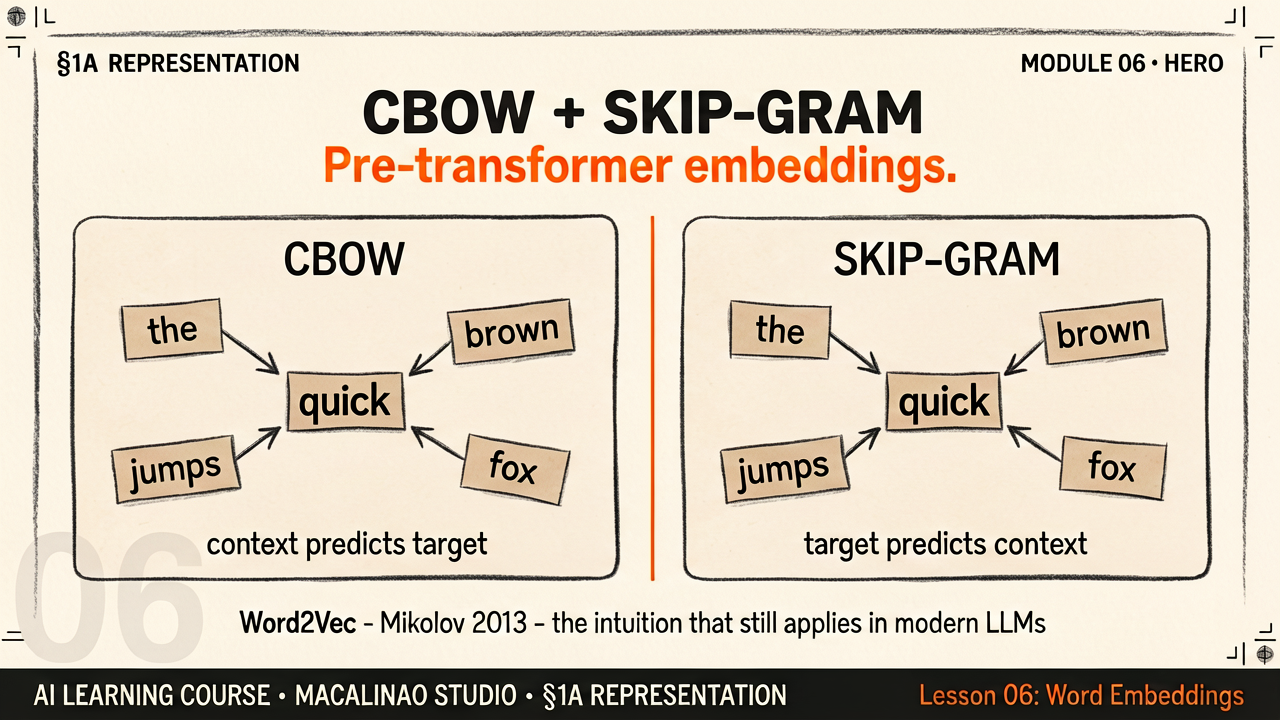
Many → One: use the surrounding words to predict the missing word
CBOW takes a window of context words around a gap and predicts what word belongs in the gap. The "bag" in the name means the order of context words doesn't matter — only their average embedding does. Training millions of these predictions forces the model to learn that similar words appear in similar contexts, which is exactly what makes embeddings useful.
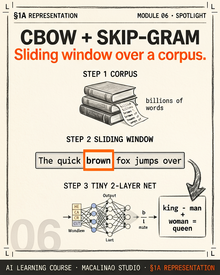
Step 1 of 5
CBOW network — context words averaged → hidden layer → predict target
How training works
For each position in the corpus, the algorithm slides a window (typically 5 words wide: 2 left + target + 2 right). The context words are embedded, averaged together, and passed through a two-layer network. The output is a probability over all vocabulary words. Loss = cross-entropy between predicted distribution and the actual target word.
Connection to BERT
BERT's Masked Language Modelling (MLM) is CBOW scaled up. Instead of a 2-word context window, BERT uses the full sentence. Instead of averaging embeddings, BERT uses deep transformer attention. Instead of a shallow network, BERT uses 12–24 transformer layers. Same idea, massively more powerful execution.
Skip-gram
One → Many: use one word to predict all its surrounding context words
Skip-gram inverts CBOW: given one input word, predict each context word in the surrounding window. For a window of ±2, each input word generates 4 training examples. This means rare words get many more training signals than in CBOW, making Skip-gram much better at learning embeddings for rare or technical vocabulary.
Step 1 of 5
Skip-gram network — input word → hidden layer → predict each context word separately
Negative sampling — the key speedup
Why training on all 50,000 words per step is impractical — and how to fix it
Without negative sampling, every training step requires computing a softmax over the entire vocabulary (50,000+ items) — enormously slow. Negative sampling instead updates weights for just the correct context word (positive) plus 5–20 randomly chosen wrong words (negatives). The model learns to distinguish real context from random noise. This makes training ~1,000× faster with minimal quality loss.
positive
"sat" (correct context)
score → high
negative ×5
"democracy"
score → low
"algorithm"
score → low
"umbrella"
score → low
Update only 6 word vectors per step instead of 50,000 — same learning signal, 1,000× faster.
CBOW vs Skip-gram — when to use each
Two algorithms, different strengths
Both CBOW and Skip-gram learn the same kind of embedding — dense vectors where similar words end up nearby. But they differ in speed, quality for rare words, and what they are optimised for. In practice, Skip-gram with negative sampling tends to produce better embeddings for most tasks, especially when rare words matter.
Property CBOW Skip-gram
DirectionContext → Target (many→one)Target → Context (one→many)
Training signals1 prediction per position2×window predictions per position
Frequent wordsBetter (smoothed by averaging)Good
Rare wordsWeakerBetter (more training signals)
Training speedFasterSlower (but still fast)
Best forLarge corpora, frequent wordsSmall corpora, rare/technical words
Modern equivalentBERT MLMContrastive learning (CLIP, SimCSE)
Context order matters?No (bag = unordered)No (predicts each separately)
What they share
Both use a two-layer neural network with no hidden-layer activation function. Both learn two embedding matrices: one for input words, one for output words. Both are trained with stochastic gradient descent. Both produce the same quality of final embeddings — the difference is in training efficiency and which words benefit most.
Window size tradeoff
Smaller window (±1–2): embeddings capture syntactic relationships — words that appear in similar grammatical positions become similar. Larger window (±5–10): embeddings capture semantic/topical relationships — words used in similar topic contexts become similar. Most Word2Vec implementations default to ±5.
Efficient Estimation of Word Representations in Vector Space (Word2Vec) — Mikolov et al., Google 2013 (arXiv:1301.3781). Introduced both CBOW and Skip-gram in a single paper. Demonstrated the vector arithmetic properties that made embeddings famous.
Distributed Representations of Words and Phrases and their Compositionality — Mikolov et al., Google 2013 (arXiv:1310.4546). Follow-up paper introducing negative sampling and subsampling of frequent words, making training practical at scale.
The embedding algorithm family tree — 1986 to 2024
Every major word representation method and how they connect
The history of word embeddings is a story of increasing expressiveness: from manually crafted features, to static vectors, to context-dependent representations, to the trillion-parameter transformers that are now the embedding layer of every frontier LLM.
1986
Distributed representations (Hinton)
First proposal that words should be represented as vectors rather than atomic symbols. Purely theoretical — no practical training at scale yet.
1990s–2000s
One-hot encoding & count matrices
Words represented as sparse binary vectors (one 1 among 50,000 zeros). Word co-occurrence matrices (LSA, PMI). Very high-dimensional, no arithmetic properties.
2013
Word2Vec — CBOW and Skip-gram (Mikolov et al.)
First practical, scalable dense embeddings. Trained on 100B words in hours. Vector arithmetic emerged: king−man+woman≈queen. The moment everyone took embeddings seriously.
2014
GloVe (Pennington et al., Stanford)
Global co-occurrence matrix factorisation. More stable training than Word2Vec. Better at capturing word analogies. Still widely used as a baseline today.
2017
FastText (Joulin et al., Meta)
Extends Skip-gram with character n-gram subwords. "running" → "run" + "unn" + "nni" + "nin" + "ing". Can represent unseen words. Essential for morphologically rich languages.
2018
ELMo (Peters et al., AI2)
First contextual embeddings. Uses a bidirectional LSTM — the same word gets different vectors depending on context. "bank" near "river" ≠ "bank" near "money".
2018
BERT (Devlin et al., Google)
Transformer-based contextual embeddings. Masked language modelling (CBOW at scale with full attention). Every token's representation depends on the full sentence. Set state of the art on 11 NLP tasks simultaneously.
2021
CLIP (Radford et al., OpenAI)
Extends contrastive learning to images. The same embedding space holds both word vectors and image vectors. Enabled text-to-image generation — words and images now in the same coordinate system.
2022–2024
Frontier LLM embeddings
The embedding layer is now a 12,288-dimensional lookup table of 100K+ tokens, trained on 15T+ tokens. The embedding algorithms of 2013 evolved into the first and last layers of every model that powers AI assistants today. CBOW and Skip-gram are inside every modern LLM — just at a much larger scale.
§ DEMO

Try it: tokenizer playground.

Type text. Watch BPE-flavored tokenization split it into chips. Compare bytes, characters, words, tokens.

Tokenizer Playground · interactiveOpen standalone
§ PAPERS

Further reading.

The canonical references for this module. External links open in a new tab.

§ NEXT

What to read next.

Use the pager below to move sequentially through the curriculum, or jump to any module from the course index. Each track has a "Prereq: ↑ foundation" callout so you can backfill anything that wasn't clear.