Training happens once — inference runs billions of times
Everything covered so far — pretraining, SFT, RLHF, GRPO — describes how a model is built. But over 90% of the total cost of running an LLM in production is inference: the forward pass that converts your prompt into a response. Every API call, every chatbot reply, every code completion is an inference request. Understanding inference is the difference between a working demo and a scalable product.
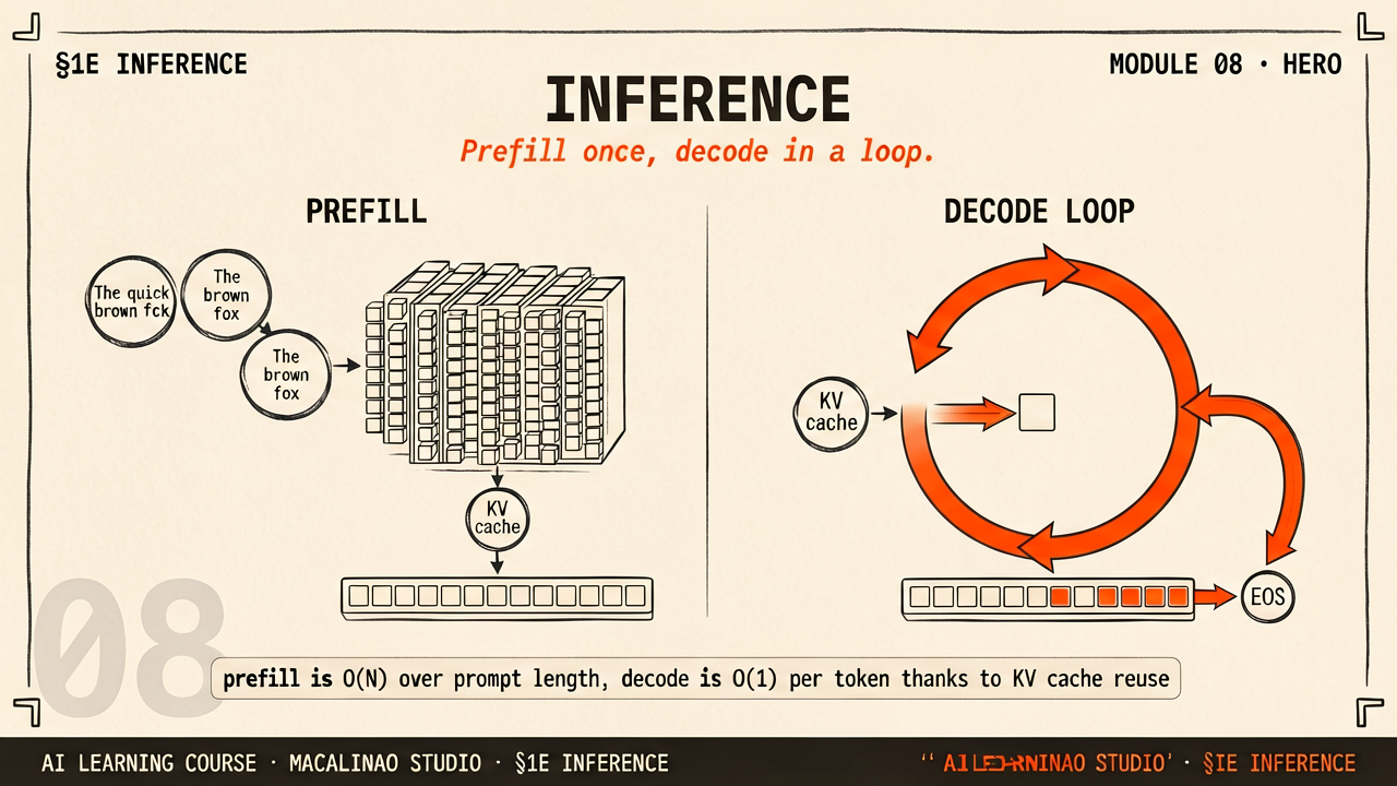
The two phases of every LLM response
Phase 1 — Prefill All prompt tokens are processed in parallel in a single forward pass. The GPU is compute-bound — doing a lot of matrix multiplications simultaneously. Builds the initial KV cache. Fast for short prompts, slow for long ones (10K+ tokens). This is why there is a slight pause before the first word appears. Phase 2 — Decode Output tokens are generated one at a time, each requiring a full forward pass. The GPU is memory-bandwidth-bound — loading model weights from memory for each step. Output tokens cost 3–10× more than input tokens. This is why streaming feels different from the initial wait.
>90%
of LLM cost is inference, not training
0–10×
output tokens cost more than input
0 token
per decode step (unless speculative decoding — see below)
The autoregressive bottleneck
Language models generate one token at a time — each new token depends on every previous token. This sequential dependency cannot be parallelised across the output sequence. A 500-token response requires 500 separate decode steps regardless of how many GPUs you have. Inference optimisation is fundamentally about making each decode step as fast and cheap as possible.
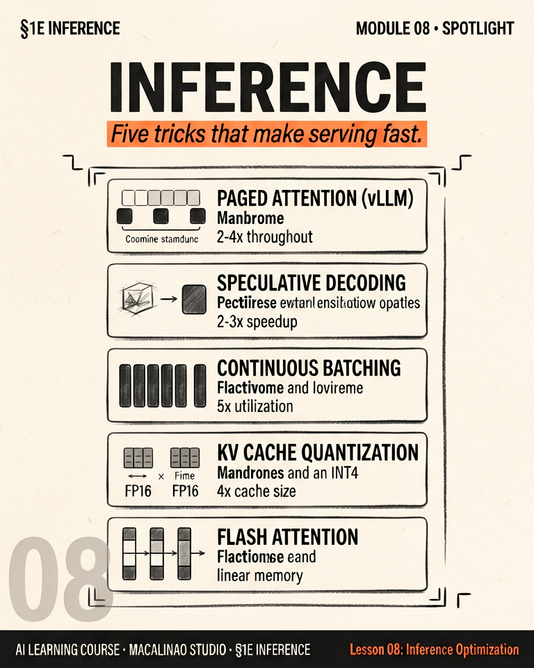
The five key techniques
KV cache — don't recompute attention for past tokens. Quantization — shrink model weights to 4-bit or 8-bit. Speculative decoding — draft multiple tokens in parallel. Continuous batching — keep the GPU busy across users. FlashAttention — fuse attention computation on-chip. Together these achieve 10–100× better throughput than naive inference.
§ 02
KV cache ★ animated
The single most important inference optimisation
KV cache — never recompute attention for tokens you've already seen
During the decode phase, each new token must attend to every previous token. Without a cache, the model recomputes the Key and Value vectors for all past tokens at every single step — an O(N²) cost. The KV cache stores these K and V vectors as they are computed, so each decode step only needs to compute new K and V for the one new token. This turns O(N²) into O(N) — a fundamental speedup.
Without cache vs with cache — attention computation per decode step
No cache (step 100): recompute K+V for all 100 past tokens + 1 new = 101 K/V computations. With KV cache (step 100): compute K/V for just the 1 new token — but attention still reads all 100 cached entries, so each step remains O(N) in memory reads. The saving is in computation: quadratic total work becomes linear.
Memory cost of the KV cache
The KV cache is not free. Every token in the context window needs to store K and V vectors for every layer. Llama 3 8B with GQA (8 KV heads): 32 layers × 2 (K+V) × 8 heads × 128 dims × 2 bytes (BF16) ≈ 0.131 MB per token. A 128K context window ≈ 17 GB of KV cache — roughly the size of the 8B model's BF16 weights themselves. With full multi-head attention (32 KV heads) it would be ~0.5 MB per token ≈ 67 GB, which is exactly why GQA exists. This is why long-context inference is so expensive.
PagedAttention & vLLM
Before vLLM (2023), KV cache memory was pre-allocated contiguously — up to 80% was wasted due to fragmentation. PagedAttention divides the cache into fixed-size "pages" (like OS virtual memory), allocating only as needed. This achieved near-zero waste and enabled much larger batch sizes, dramatically cutting cost per token in production.
§ 03
Quantization
Quantization — shrinking the model without breaking it
Models trained in 16-bit can be served in 4-bit — with minimal quality loss
A model's weights are floating-point numbers. During training they use BF16 or FP16 (16 bits each). Quantization converts these to lower-precision formats: INT8 (8 bits) or INT4 (4 bits). The result: half or quarter the memory, and faster matrix operations on hardware that supports lower-precision arithmetic. The decode phase is memory-bandwidth-bound — reading weights is the bottleneck — so 4-bit weights can be read up to 4× faster than 16-bit.
Memory savings across precision formats — Llama 3 70B
FP32 (full precision) 280 GB — needs 4+ A100 GPUs BF16 (training default) 140 GB — 2 A100s INT8 70 GB — 1 A100 INT4 (4-bit) 35 GB — a Mac with unified memory, or 2 consumer GPUs
GPTQ — post-training quantisation
GPTQ quantizes a model after training with no retraining required. It uses a second-order method to compensate for quantization error layer by layer, finding the INT4 weights that minimize the change in output. Achieves near-FP16 quality at INT4 precision. The GPTQ lineage lives on in ExLlama (EXL2 format); GGUF/llama.cpp use their own block-wise k-quant and i-quant schemes, not GPTQ.
AWQ — activation-aware quantisation
AWQ (Lin et al. 2024) observes that not all weights are equally important — a small fraction of weights (those connected to large activation values) contribute disproportionately to the model's output. AWQ identifies and protects these "salient" weights from aggressive quantization while compressing the rest. Achieves better quality than GPTQ on most tasks at the same bit width. vLLM supports it but applies no quantization by default — it serves BF16 unless asked. In 2026 production the most common served format is FP8 W8A8 — weights, activations, and KV cache all in FP8. DeepSeek's multi-head latent attention (MLA) attacks the same memory problem at the architecture level, compressing K/V into a low-rank latent.
The outlier problem — why quantization is hard
Activation outliers are the main challenge
Weights are easy to quantize — they are fixed after training and can be analyzed carefully. Activations are harder — they change with every input and often contain a few very large "outlier" values. A single outlier at value 1,000 in an INT8 range forces the entire activation to be scaled to fit, wasting most of the precision on near-zero values. LLM.int8() (Dettmers 2022) solved this by separating outlier dimensions and keeping them in FP16 while quantizing the rest to INT8 — the first method to achieve good INT8 inference quality on large models.
§ 04
Speculative decoding
Speculative decoding — generate multiple tokens for the cost of one
A small draft model guesses ahead — the large model verifies in parallel
The core problem with autoregressive decoding: the large model must run once per output token. Speculative decoding sidesteps this by using a small, fast draft model to generate k candidate tokens (typically 3–7). The large "target" model then verifies all k tokens in a single parallel forward pass — the same computation as generating one token normally. If the draft was correct, you get k tokens for the cost of 1. If not, you fall back to the target model's correction.
Why this works
Verifying k tokens in the large model costs the same as generating 1 token — both process k+1 positions in a single forward pass. On tasks where the draft model is accurate (code completion, factual text), acceptance rates of 70–90% are common, meaning you effectively get 3–5 tokens per large model step instead of 1. Speedups of 2–4× are typical for coding tasks.
Draft model choices
Separate small model: A 1–7B model drafts for a 70B model. Works well for general text. EAGLE / Medusa: A lightweight head on the target model itself drafts future tokens using the hidden states — no separate model needed. n-gram lookup: Ultra-fast draft using repeated phrases from context. Great for code with repetitive patterns. Supported in vLLM (not enabled by default).
0–4×
typical speedup for coding tasks
0–90%
token acceptance rate on domain tasks
k=4
typical draft length (3–7 tokens)
§ 05
Batching & serving
Serving LLMs at scale
Continuous batching — keep the GPU busy across hundreds of users
A GPU is only efficient when it is processing many requests simultaneously. Early LLM servers used "static batching" — wait for a full batch of N requests, process them all together, then wait again. The problem: requests finish at different times, leaving the GPU idle while waiting for the slowest request. Continuous batching (also called iteration-level batching or in-flight batching) inserts new requests as soon as any sequence completes — keeping GPU utilisation near 100% continuously.
The complete inference optimisation stack
KV cache + PagedAttention Never recompute past attention. Allocate cache memory like OS virtual memory — near-zero waste. Prerequisite for everything else.
Inference engines in production
vLLM — PagedAttention + continuous batching; the open-source default with the broadest model support. UC Berkeley lineage.
TensorRT-LLM — NVIDIA's compiled-kernel engine; trades build time for peak per-GPU throughput on NVIDIA hardware.
Structured outputs (JSON-schema-constrained decoding) are now a standard serving feature in all three, and reasoning models have made decode-heavy workloads the dominant inference cost.
Prefix caching
If many requests share the same prefix — a long system prompt, the same RAG document, the same code file — you can compute the KV cache for that prefix once and reuse it for all users. Prefix caching eliminates up to 90% of prefill cost for workloads with shared context. Standard in SGLang (RadixAttention), vLLM (hash-based), and Anthropic's prompt caching API.
§ 06
The playground.
Theory above, instrument below. This interactive panel runs live in the page — drag, type, and watch the mechanism respond.