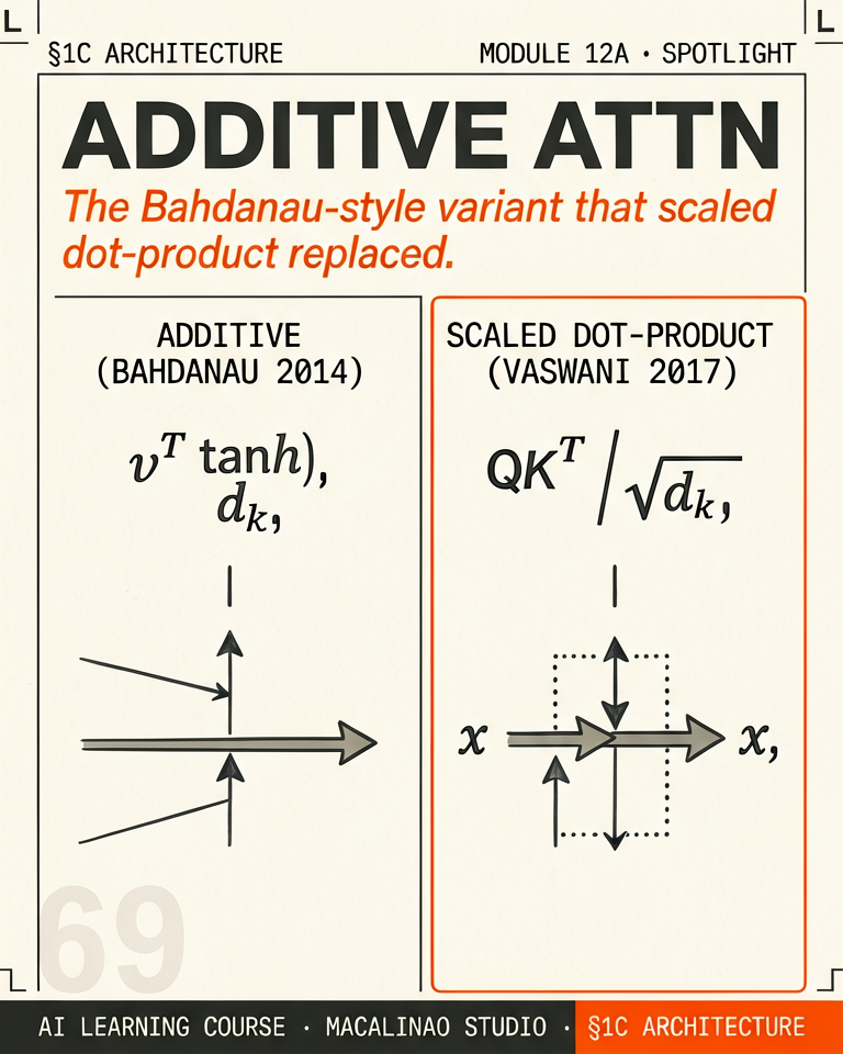
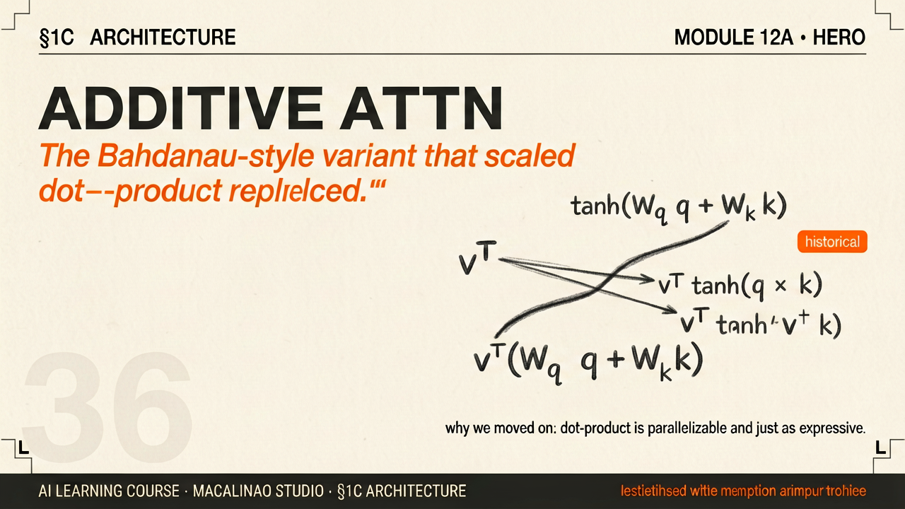
Narration · Module 12a
Additive Attn
0:00 / 0:00
Module 12a · Architecture · 5 min

Additive attention,
briefly.

The Bahdanau-style variant that scaled dot-product replaced.

Reading time5 min Audionarration available Prerequisites12 SourceTrack A · Gemini
§ 1

What this lesson covers.

This module is one of 42 in the curriculum. Below is the canonical interactive lesson — tabs, cards, and diagrams from the source repo, rendered inside the course shell. An audio narration runs alongside it - the sticky player at the top of the page plays the full Module 12a clip.

If you prefer to read first and play with the demos after, the interactive lesson sits below this section. If you'd rather hear it narrated while you scroll, hit play on the sticky audio bar at the top — or just let it autoplay.

§ 2

The lesson itself.

Interactive lesson · ported from Gemini track Click tabs to navigate · hover cards for details

Attention Mechanism — The Heart of Every Transformer

Self-attention · Q·K·V · Causal masking · Multi-head · FlashAttention · Layer 3

Layer 3 — Attention
The big idea
Attention lets every word look at every other word and decide what matters
Before attention, neural networks processed words one at a time — each word only "saw" its immediate neighbours. This broke down for long-range dependencies like "The trophy didn't fit in the suitcase because it was too big" — where "it" could refer to either noun. Attention solves this by letting "it" directly compare itself to every other word simultaneously and decide which one is most relevant. This happens inside every single transformer block, at every layer, for every token.
Step by step — what attention computes
1 / 7
O(N²)
Attention is quadratic in sequence length — the main scaling challenge
32 heads
Llama 3 70B runs 32 parallel attention heads per layer
128K
Maximum context window — tokens that can attend to each other simultaneously
Before attention — RNNs
Recurrent Neural Networks processed words one at a time, left to right. Information about early words had to pass through every subsequent step — like a game of telephone. By the time a 500-word document reached its end, the RNN's memory of the opening sentences was severely degraded. Long-range dependencies were nearly impossible.
After attention — Transformers
Attention computes relationships between ALL pairs of tokens simultaneously — in parallel. Word 1 can directly attend to Word 500. The distance between words is irrelevant. This is why transformers can handle documents, books, and eventually 128K+ token contexts — the architecture has no inherent concept of "too far away."
Attention Is All You Need — Vaswani et al., Google Brain 2017 (arXiv:1706.03762). Introduced the transformer with scaled dot-product attention. Eliminated recurrence entirely. 90,000+ citations — one of the most influential papers in ML history.
FlashAttention: Fast and Memory-Efficient Exact Attention — Dao et al. 2022 (arXiv:2205.14135). Rewrote the attention computation using IO-aware tiling. 2–4× speedup, dramatically reduced memory. Standard in all frontier model training and inference.
Interactive attention heatmap
Click any word — watch what the model attends to
Each cell shows how much attention the query word (row) pays to the key word (column). Brighter = more attention. These weights are learned — not hardcoded. A real transformer would produce different patterns depending on the layer and head. The patterns below are illustrative but grounded in empirically observed attention behaviour.
Click a word to set it as the query — see its full attention distribution
Sentence:
Attention weight:
0.00.51.0
What makes a pattern meaningful
Syntactic heads learn grammatical relationships: a verb attending to its subject, a pronoun attending to its antecedent. Semantic heads learn meaning relationships: "Paris" attending to "France." Positional heads learn position: each token attending mostly to the previous token. A 32-head model has 32 specialised perspectives running simultaneously.
Not all heads are equal
Research shows that in large models, a small fraction of attention heads do most of the "interesting" work — handling coreference, syntax, and factual associations. Many heads appear to learn near-trivial patterns. This has motivated pruning research: removing 20–40% of attention heads from BERT causes minimal quality loss.
Query · Key · Value
Three linear projections — Q asks, K answers, V delivers
Every token's embedding is projected through three separate learned weight matrices to produce three vectors: the Query (what am I looking for?), the Key (what do I contain?), and the Value (what information do I carry?). The dot product of Q and K gives a relevance score. Softmax converts scores to weights. The weighted sum of V vectors is the output. Drag the sliders below to feel how each dimension affects the attention score.
Live QKV playground — drag Q and K vectors, watch the score update
Query vector Q (4 dims)
Key vector K (4 dims)
Raw dot product Q·K
0.00
÷
Scale √d_k (d=4)
2.00
=
Scaled score
0.00
Softmax → attention weight (vs 3 other tokens)
25%
Why scale by √d_k?
Without scaling, softmax saturates and gradients vanish
With high-dimensional vectors (d=512, 1024, 4096), the dot product Q·K grows proportionally to √d. A dot product of 50 vs 55 produces very different softmax outputs than a dot product of 5 vs 5.5. At large d, the scores become so large that softmax essentially puts all weight on the maximum — almost a hard argmax. This makes gradients near zero for non-maximum positions. Dividing by √d_k keeps scores in a regime where softmax behaves smoothly.
The Value vector's role
Q and K determine HOW MUCH to attend to each position. V determines WHAT information to extract from each position. They are separate projections so the model can learn different representations for "this is what I am" (K) vs "this is what I send" (V). This separation is what gives attention its expressiveness — a token can say "I am highly relevant to your query" (high K·Q) but carry completely different information in V.
Learned projections
W_Q, W_K, W_V are all learned weight matrices. In GPT-3 (d=12288, 96 heads, d_head=128): each of Q, K, V is shape [12288, 128] — that is 4.7M parameters per head just for projections. With 96 heads across 96 layers, attention projections alone account for billions of parameters. These weights are what the model learns during training — not the attention patterns themselves.
Causal masking
Decoder-only models can only look backwards — never forwards
In a language model that generates text left-to-right, a token cannot use future tokens to predict itself — that would be cheating. The causal mask enforces this by setting all future attention scores to −∞ before the softmax. After softmax, e^(−∞) = exactly 0 — so future positions receive precisely zero attention weight. This mask is applied during every training step so the model learns to predict each token from only previous context.
Interactive causal mask — hover each cell to understand it, toggle bidirectional mode
Current: causal (decoder-only)
Hover any cell to see what it means
Can attend (past/self)
Masked (future = −∞)
Bidirectional mode
Why −∞ and not 0?
If you set masked positions to 0, then e^0 = 1 — they still contribute a non-zero weight after softmax. Using −∞ means e^(−∞) = 0, giving exactly zero weight. This is mathematically precise and computationally efficient. In practice, implementations use a very large negative number like −10,000 rather than true −∞ to avoid NaN values in floating point arithmetic.
Encoder vs decoder masking
BERT-style encoders use bidirectional attention — no causal mask. Every token attends to every other token. This is why BERT cannot generate text: it needs future tokens to compute its representations. GPT-style decoders use the causal mask — each token only attends backwards. This is the architectural difference that makes GPT able to generate and BERT unable to.
Training efficiency: teacher forcing
The causal mask enables training on all positions simultaneously
At training time, we know the entire correct sequence. The causal mask lets the model compute predictions for all positions in one forward pass, in parallel — using the correct previous tokens as context (not the model's own predictions). This is called "teacher forcing." Without the causal mask, you would have to process each position sequentially. With it, training is massively parallelised across the entire sequence length.
Multi-head attention
Run attention in parallel with different "perspectives" — each learning something different
Instead of one attention computation, multi-head attention runs h parallel attention operations ("heads"), each with its own learned Q, K, V projections. Each head learns to attend to a different type of relationship — some heads specialise in syntax, some in semantics, some in position, some in coreference. Their outputs are concatenated and projected back to the original dimension.
Multi-head visualiser — click a head to see its specialisation
How the heads combine
head₁ head₂ head₃ … headₕ → concat → [head₁; head₂; … headₕ] × W_O → output
Each head produces d_head dimensional output. h heads concatenated = h × d_head = d_model total. The output projection W_O mixes information from all heads into the final representation.
Grouped Query Attention (GQA)
Modern models (Llama 3, Mistral) use GQA: multiple Query heads share a single Key+Value head. Llama 3 70B: 64 Q heads, 8 KV heads — each KV head is shared by 8 Q heads. This reduces the KV cache size by 8× at inference time with minimal quality loss, making 128K+ context windows practical.
Multi-Query Attention (MQA)
The extreme version: all Q heads share one K+V pair. Used in Falcon and early Gemini. Even smaller KV cache — but can hurt quality for tasks requiring diverse attention patterns. GQA (used in Llama) is the compromise: groups of Q heads sharing KV, offering most of the memory benefit with less quality loss.
The complete attention formula
Everything in one equation — and what each part does
The full scaled dot-product attention formula is deceptively compact. Every element has a precise reason for being there. Walk through it component by component using the stepper below.
Attention(Q,K,V) = softmax( Q·Kᵀ / √dk + M ) · V
Q = query matrix K = key matrix V = value matrix M = mask (causal or none) d_k = head dimension
Step through each component
1 / 7
Connections to the rest of the curriculum
→ Layer 6: Output head
The softmax in attention weights Values. The softmax in the output head (Layer 6) selects the next token. Same operation, completely different purpose — one weights information, one picks a word.
→ Layer 7: KV cache
The K and V matrices for all past tokens are cached at inference time. Each new decode step only computes K and V for the one new token — everything else is reused from cache. This is why inference is O(N) not O(N²).
→ Layer 1: Positional encoding
RoPE (used in Llama 3) works by rotating the Q and K vectors before the dot product. The rotation angle encodes position, so Q·K naturally captures relative distance. Position is baked into the attention computation itself.
→ Layer 4: Transformer block
Attention is one sublayer inside the transformer block. After attention: Add & Norm (residual + LayerNorm), then the Feed-Forward Network, then another Add & Norm. The attention output is added to the input (residual), not replacing it.
Attention Is All You Need — Vaswani et al. 2017 (arXiv:1706.03762). Section 3.2 defines scaled dot-product attention and multi-head attention. The formula has not changed in 8 years.
GQA: Training Generalised Multi-Query Transformer Models — Ainslie et al., Google 2023 (arXiv:2305.13245). Introduced Grouped Query Attention. Now standard in Llama 3, Mistral, Gemma.
§ PAPERS

Further reading.

The canonical references for this module. External links open in a new tab.

§ NEXT

What to read next.

Use the pager below to move sequentially through the curriculum, or jump to any module from the course index. Each track has a "Prereq: ↑ foundation" callout so you can backfill anything that wasn't clear.